ERA5 reanalysis

We used the hourly ERA5 reanalysis (Hersbach et al., 2020) with its original horizontal resolution of 0.25°, or about 31 km, for its near real time availability from 1950 to the present as a benchmark to develop the gridded dataset of variables and indices, including the FWI System components, across Canada.

ERA5 reanalysis was provided by ECMWF (European Centre for Medium-Range Weather Forecasts) and accessed via the Climate Data Store (C3S, 2025) download platform. This fifth-generation reanalysis was developed by the ECMWF center via assimilation with the 4D-VAR method of satellite observations and in situ meteorological data collected by the World Meteorological Organization (WMO; Hersbach et al., 2020). Access to the most recent ERA5 data, commonly referred to as ERA5T (see C3S, 2025), is limited to six days before the current day. Therefore, if the current day is July 10, the latest available data for download dates to July 3, necessitating a six-days lag.

CRCM6-GEM5

In the near future, we plan on adding a section on the changes in the FWI System components under climate change. This will be done using high resolution (12 km) simulations from the new Canadian regional climate model (CRCM version 6, i.e. CRCM6 used and described in Llerena et al., 2023, and Roberge et al., 2024), developed at ESCER (UQAM). CRCM6 is based on the HRDPS (High Resolution Deterministic Prediction System) model and GEM5 physics (McTaggart et al., 2019).

Data for validation

The latest FWI values calculated by the Canadian Wildland Fire Information System from observation station data (CWFIS-FWI), are used for comparison with daily FWI values calculated using ERA5. Nearly 650 CWFIS meteorological stations across Canada are available on average, depending on the day.

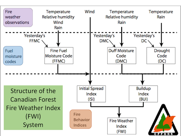
Overview of the Canadian Forest Fire Weather Index (FWI) System calculation

The FWI System is composed of three fuel moisture codes, i.e., the Fine Fuel Moisture Code (FFMC), the Duff Moisture Code (DMC) and the Drought Code (DC), as well as three fire behavior indices, i.e., the Initial Spread Index (ISI), the Buildup Index (BUI) and the Fire Weather Index (FWI), calculated on a daily basis (Fig. 1). Their calculation requires the following fire weather observations at local standard noon (following the standard UTC method, see Van Wagner and Pickett, 1985):

• Air temperature at 2-meters above ground (in °C);
• Relative humidity at 2-meters above ground (in %);
• Wind speed at 10-meters above ground (in km h-1); and
• Accumulated precipitation over the last 24 hours (in mm).

• Previous day's FFMC (start-up default value is 85);
• Previous day's DMC (start-up default value is 6); and
• Previous day's DC (start-up default value is 15).

FWI System calculation using the solar noon method

We developped the solar noon (SN) method for FWI System calculation to provide fire weather data based on a more "physical" approach compared to the classical approach (UTC method). The UTC method uses fire weather readings at local standard noon which results in arbitrarily assigned values based on common longitudes and not dependent on the seasonal cycle. In contrast, the SN method is based entirely on the property of the sun's elevation above the local horizon, i.e., the local insolation conditions. The SN method also solves temporal biases and artifacts associated with the UTC method across time zones, thus allowing for a more homogeneous and spatially continuous field along time zone boundaries and across longitudes over Canada using medium– to fine–scale gridded data.

To calculate the FWI System components using the SN method, we selected the input fire weather parameters at the time corresponding to when the sun reaches the local meridian (i.e., the highest position of the sun in the sky) for each grid point and for each day. Local solar noon at each location on Earth’s surface was determined following Duffie et al. (2020). A longitude correction was first applied to the local time (1° of longitude corresponds to a time difference of 4 minutes). A correction called the "equation of time" was then applied, which corresponds to the fact that the Earth does not always move at the same speed on its orbit, so the sun can appear at the zenith with a deviation of up to ±16 minutes compared to the local time or UTC.

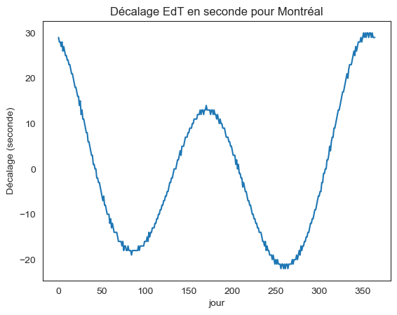
The calculation of solar noon was performed using the Python library "daylight" (Python Package Index - PyPI, 2020) which allows the obtention of the solar noon time in UTC from geographic coordinates. Since the meteorological variables from the ERA5 reanalysis are provided on an hourly basis Coordinated Universal Time (UTC), the local solar noon corresponding value for each variable was calculated using a temporal proximity proportion or weighted average value that was applied between the two temporally closest fields. For example, if for a grid point the solar noon of the day was calculated at 18:20 UTC, the field value had to be weight-averaged using the 18:00 UTC and 19:00 UTC fields using 2/3 and 1/3 as the respective weights. This technique allows for a spatially explicit calculation of the various indices that eliminate artifacts along time zone boundaries across Canada.

We used a Python code composed of six functions that we derived from the fwi function of the Canadian Forest Fire Danger Rating System (cffdrs) R library (Wang et al., 2024). This library was developed to calculate fire danger indices for single meteorological stations and was therefore adapted for model data or gridded data in NetCDF format, in Python programming language. In addition to the six FWI System outputs, we calculated the Daily Severity Rating (DSR), which is a numerical assessment of the difficulty or effort expected to control fires, as well as the cumulative DSR over each fire season (DSRc), which gives a relevant indication of fire severity over an entire season.

An automated daily FWI values comparison has been developed with the FWI calculated from the CWFIS observation station data network (see the latest comparison here : FWI).

Overwintering adjustment of the DC

In Canada, it is assumed that FFMC and DMC reach the moisture saturation point of winter precipitation at the time of spring melt. This assumption is reasonable because the assumed initial conditions disappear rapidly after a few days. However, due to the relatively long response time of the DC fuel layer (around 53 days under normal conditions), any bias in the estimation of this starting condition before the arrival of spring or thawing conditions can affect the DC at the beginning of the fire season (Hanes et al. 2020). If the fuel layer required for the DC calculation does not fully reach saturation when the snow melts in the spring, an overwintering adjustment of the DC start-up value needs to be applied, which is often the case in the dry areas of the Canadian Prairies (de Groot et al., 2015). At each year's start-up date, we applied the overwintering procedure of the DC for the regions where the last DC value from the previous fire season (DCf) was far from saturation, i.e., ≥ 50, following Hanes and Wotton (2024), and used start-up default value of 15 elsewhere.

• DC moisture equivalent at the end of fall (Qf):

\(\text{Qf} = 800 \times \exp(\frac{-\text{DCf}}{400})\)



• DC moisture equivalent at the beginning of spring (Qs):

\(\text{Qs} = a \times Qf + b \times (3.94 \times rw)\)



• DC obtained for the beginning of the fire season (DCs):

\(\text{DCs} = 400 \times log(\frac{800}{Qs})\)

We used a value of 1.0 for the carry-over fraction (a) and a value of 0.5 for the wetting efficiency fraction (b), as suggested by Hanes and Wotton (2024). The accumulated precipitation during winter (rw) was calculated, locally, from the day following the end of the previous fire season to the next fire season onset.

Calculation of the start and end of the fire season

By convention, the FWI System calculations are stopped at the end of the fire season and are restarted the next spring, on onset day, using the start-up default values for FFMC, DMC and DC components.

We defined the end of the fire season (WinterOnset) following the approach outlined by Wotton and Flannigan (1993), as the fourth day following three consecutive days with daily maximum temperature (tasmax) < 5°C.

For the calculation of the start of the fire season (Onset), we considered both temperature and snow conditions. In snow-covered regions, the initiation of the calculation in the spring is scheduled to start the first day of the year following three consecutive days with no snow cover and with tasmax greater than 12°C while it is scheduled to occur the first day of the year following three consecutive days with tasmax greater than 12°C for non-snow-covered regions, according to Turner and Lawson (1978). Snow-covered regions are defined as regions where at least 75% of the days in January and February have a mean snow depth value of 0.10 m or greater (CWFIS, n.d.).

However, we found that using ERA5 reanalysis data was leading to important delays in ablation of snowpack in the spring, that did not correspond to the ablation date given by satellite observation data, especially in the Rocky Mountains or surrounding areas (see Appendix A, Fig. A1), which was also mentioned in other studies (Kouki et al., 2023; Lei et al., 2023; Hersbach et al., 2020). Moreover, during data preparation and exploration phase, we found that some grid points in mountainous areas (Rocky Mountains for example) would never show 3 consecutive days with a snow depth value of 0 meter for some years, which was again inconsistent with satellite-based observations.

We therefore adapted the methodology for calculating onset using ERA5 data, utilizing temperature and snow conditions, with a snow depth threshold set at 0.01 meters ("TS" method). We found that using this threshold value instead of 0 meter, would lead in a more accurate onset date. Snow conditions were verified using the daily mean snow depth (sdmean) and no onset was calculated for regions where sdmean never reaches values below 0.01 meters.

Spatial scales of analysis

Analysis are carried out at 2 spatial scale levels:

1. ERA5 cell-level analysis
   Analyses at high spatial resolution, carried out at the original grid resolution of the ERA5 reanalysis (~31 km) and where values are represented for each grid point covering all of Canada's landmass;
2. Territories-level analysis
   Analyses that summarize variables and indices in the form of spatial statistics (spatial median, for example) at the scale of the following predetermined territories:
1. The landmass of Canada
2. Each province of Canada
3. Each terrestrial ecozone of Canada*
4. Each SOPFEU protection zones (for Quebec only)

*Canada's terrestrial ecozones are defined by the National Ecological Framework for Canada (cf. Ecological Stratification Working Group, 1996) and represent the highest of four levels of ecosystem classification. In all, fifteen terrestrial ecozones subdivide Canada, representing the country's major ecological units in a highly generalized manner. These units are characterized by constantly interacting and adapting biotic and abiotic factors (Wiken, S.D.; for more details, see Wiken 1986). Ecozones have been redefined, in some cases, according to the boundaries of ecoprovinces (the second level of ecosystem classification) in order to obtain more homogeneous sectors in terms of their longitudinal extent.

Daily Analysis

Interactive Meteograms

Periodic Analysis

Absolute value maps

Anomaly maps

The absolute, relative and standardized interannual anomalies of the different monthly, seasonal and annual variables and indices are calculated as follows

Absolute anomaly:

Relative anomaly:

Standard anomaly:

Where \(\text{Xi}\) is the value for the year of interest, \(\text{Xi_clim}\) is the climatological average over the reference period from 1991 to 2020 and \(\text{Xi_std}\) is the standard deviation over the reference period from 1991 to 2020.

All anomalies are calculated with respect to the most recent climatology (1991 to 2020 period). The absolute anomaly (Equation 1) is given in the same units as the variable or index studied, the relative anomaly (Equation 2) is given in percent, and then the standardized anomaly (Equation 3) is given in standard deviations. The standardized anomaly (Equation 2) is better able to account for the extreme or atypical nature of the observation (International Research Institute for Climate and Society (IRI), 2020) and allows comparison of anomalies between variables or indices, regardless of the variability of the variable itself.

Anomalies for most monthly weather indices and variables are calculated and plotted as 1 km resolution maps over the entire BVRO using Daymet data, for the months of March, April, and May 2017 and are also calculated for seasonal indices. Index values averaged over the entire BVRO, including standardized hydrologic index anomalies at the Carillon power plant, are also plotted as histograms for the months of March, April, and May of all years of interest, including seasonal indices.

Trends and Normals

Trends

The trend analysis are performed over different periods, recognizing that temperature increases have accelerated over the last three decades on a global scale (WMO, 2021). It is therefore of interest to analyze whether more recent changes (last 3 decades) are underway compared to trends covering the whole of the last 70 years.

The methodology employs the non-parametric Mann-Kendall (MK) test (Mann, 1945; Kendall, 1948) modified by a three-step approach proposed by Douglas et al. (2000) and Khaliq et al. (2008), where autocorrelations within the time series are first "pre-whitened" (von Storch 1995; Kulkarni and von Storch, 1995). The python library pymannkendall (version 1.4.1) which proposes a test using the latter methodology is used.

We calculate the Theil-Sen slope estimator with a 95% statistical significance level (p-value ≤ 0.05) for each ERA5-level cell. Test is applied only if there is data (non-NaN) for at least 30 years.

Maps show the slope values over a 10-years period (Theil-Sen slope estimator multiplied by 10). Dashes are used to mask values that are not statistically significant.

Normals

An atmospheric block is a meteorological situation often associated with a persistent area of high pressure, where the zonal west-east flow is temporarily suppressed and replaced by a meridional flow. Some atmospheric blocks, more continental in summer than in winter, take place and can be associated with the occurrence of heat waves, as was the case in June 2021 in western Canada.

In order to better understand the influence of atmospheric blocks on fire-weather indices and, more generally, on meteorological variables on the ground, a system for monitoring these blocks has been developed to identify and estimate the properties (duration, intensity, extent) of past and current blocks. This day-by-day monitoring of blockings has been carried out with the ERA5 reanalysis for the period 1950 to today, using the geopotential height at 500 hPa.

Atmospheric blocking detection follows the prerequisites of Tibaldi and Molteni, 1990, with automation modifications by Wiedenmann, 2002. In addition to identifying the presence of an atmospheric blocking center, the extent, shape, and intensity of the blocking were evaluated from its center, applying a seasonally varying amplitude threshold based on a daily climatological mean whose variability was filtered using the method of Miller et al, 2020.

All the code written in python, is fully automated every day at 2am (Montreal time). It automatically retrieves the latest data from ERA5 (about 6 days difference with the current day)

1. Canadian Forest Service: Tables for the Canadian Forest Fire Weather Index System, 4th ed., Environ. Can., Can. For. Serv., Ottawa, Ont, For. Tech. Rep. 25, 48 pp., 1984.

2. Canadian Wildland Fire Information System (CWFIS): Data Sources and Methods. Natural Resources Canada. https://cwfis.cfs.nrcan.gc.ca/background/dsm/fwi, n.d.

3. Copernicus Climate Change Service (C3S), ERA5: Fifth generation of ECMWF atmospheric reanalyses of the global climate. Copernicus Climate Change Service Climate Data Store (CDS), (2017), Site du centre ECMWF

4. de Groot W.J., Wotton B.M. and Flannigan M.D., Wildland re danger rating and early warning systems,chapter 11, pp. 207-228. Elsevier, Amsterdam, NL. (2015)

5. Douglas, E., Vogel, R., Kroll, C., Trends in foods and low fows in the United States: impact of spatial correlation, J Hydrol, 240(1–2):90–105, (2000)

6. Duffie, J. A., Beckman, W. A., and Blair, N.: Solar Engineering of Thermal Processes, Photovoltaics and Wind, Fifth Edition, John Wiley & Sons, Inc., https://doi.org/10.1002/9781119540328, 2020.

7. Hanes, C., Wotton, M., Woolford, D. G., Martell, D. L., and Flannigan, M.: Preceding Fall Drought Conditions and Overwinter Precipitation Effects on Spring Wildland Fire Activity in Canada, Fire, 3(2), 24. https://doi.org/10.3390/fire3020024, 2020.

8. Hanes, C. and Wotton, M.: Updated guidance for the Drought Code overwintering adjustment, Can. Wildland Fire Smoke Newsl., Can. Wildfire, 2–8, 2024.

9. Hersbach, H. et al, The ERA5 global reanalysis, Q. J. R. Meteorol. Soc. https://doi.org/10.1002/qj.3803., (2020)

10. International Research Institute for Climate and Society (IRI), Climatologies and Standardized Anomalies, Site de l'IRI (2020)

11. Kendallm M.G., Rank correlation methods, Grifn, Oxford, (1948)

12. Khaliq M.N., Ouarda T.B.M.J., Gachon P. and Sushama L., Temporal evolution of low-fow regimes in Canadian rivers, Water Resour Res, 44(8):W08436. https://doi.org/10.1029/2007WR006132, (2008)

13. Khaliq, M.N. et al, Identification of hydrological trends in the presence of serial and cross correlations: A review of selected methods and their application to annual flow regimes of Canadian rivers, Journal of Hydrology, 368:117-130, (2009)

14. Kouki, K., Luojus, K., and Riihelä, A.: Evaluation of snow cover properties in ERA5 and ERA5-Land with several satellite-based datasets in the Northern Hemisphere in spring 1982–2018, The Cryosphere, 17(12), 5007–5026. https://doi.org/10.5194/tc-17-5007-2023, 2023.

15. Kulkarni A, von Storch H, Monte Carlo experiments on the efect of serial correlation on the Mann Kendall test of trend, Meteorol Z, 4(2):82–85, (1995)

16. Lawson, B.D. and Armitage, O.B.: Weather Guide for the Canadian Forest Fire Danger Rating System, Nat. Res. Can., Can. For. Serv., Edmonton, Alta., 84 pp., 2008

17. Lei, Y., Pan, J., Xiong, C., Jiang, L., and Shi, J.: Snow depth and snow cover over the Tibetan Plateau observed from space in against ERA5: matters of scale, Clim. Dynam., 60, 1523–1541, https://doi.org/10.1007/s00382-022-06376-0, 2022.

18. Mann H.B., Nonparametric tests against trend, Econom J Econom Soc, 13(3):245–259, (1945)

19. McElhinny, M, Justin F. Beckers, Chelene Hanes, Mike Flannigan, and Piyush Jain, A high-resolution reanalysis of global fire weather from 1979 to 2018 – overwintering the Drought Code, Earth Syst. Sci. Data, 12, 1823–1833, (2020)

20. McTaggart-Cowan, R., Vaillancourt, P. A., Zadra, A., Chamberland, S., Charron, M., Corvec, S., Milbrandt, J. A., Paquin-Ricard, D., Patoine, A., Roch, M., Separovic, L., & Yang, J., Modernization of Atmospheric Physics Parameterization in Canadian NWP, Journal of Advances in Modeling Earth Systems, 11(11), 3593–3635. https://doi.org/10.1029/2019MS001781, (2019)

21. Miller, R.L., Lackmann, G.M. and Robinson, W.A., A New Variable-Threshold Persistent Anomaly Index: Northern HemisphereAnomalies in the ERA-Interim Reanalysis, American Meteorological Society, 43-62. https://doi.org/10.1175/MWR-D-19-0144.1, (2020)

22. Python Package Index – PyPI: daylight 0.1.3 [code]. https://pypi.org/project/daylight/, 2020.

23. Tibaldi, S. and Molteni, F., On the operational predictability of blocking, Geophysical Research Letters, 42(3):343-365. https://doi.org/10.1034/j.1600-0870.1990.t01-2-00003.x, (1990)

24. Turner, J.A. and Lawson, B.D.: Weather in the Canadian Forest Fire Danger Rating System, A user guide to national standards and practices, Environment Canada, Pacific Forest Research Centre, Victoria, BC. BC-X-177, 1978.

25. Van Wagner, C.E., Pickett, T.L., Equations and FORTRAN program for the Canadian Forest Fire Weather Index System,Canadian Forestry Service, Petawawa National Forestry Institute, Chalk River, Ontario. Forestry Technical Report 33. 18 p., (1985)

26. Van Wagner, C.: Development and structure of the Canadian Forest Fire Weather Index System, Paper presented at the Can. For. Serv., Forestry Tech. Rep., https://ostrnrcan-dostrncan.canada.ca/handle/1845/228434, 1987.

27. Von Storch, H., Misuses of statistical analysis in climate research.In: von Storch H, Navarra A (eds) Analysis of climate variability: applications of statistical techniques, Springer, Berlin, pp 11–26, (1995)

28. Wang, Y. et al, Updated source code for calculating fire danger indices in the Canadian Forest Fire Weather Index System, RNCAN, (2015)

29. Wang, X., Cantin, A., Parisien, M.-A., Wotton, M., Anderson, K., Moore, B., Schiks, T., and Flannigan, M.: Canadian Forest Fire Danger Rating System, v1.9.0, https://r-forge.r-project.org/projects/cffdrs/, 2024.

30. Wiedenmann, J. M., Lupo, A. R., Mokhov, I. I., & Tikhonova, E. A., The Climatology of Blocking Anticyclones for the Northern and Southern Hemispheres: Block Intensity as a Diagnostic, Journal of Climate, 15(23), 3459-3473, (2002)

31. WMO, The State of the Global Climate 2020., Rapport du WMO 2020, (2021)

32. Wotton, M. and Flannigan, M., Length of the fire season in a changing climate, Forestry Chronicle, 69(2):187-192, (1993)

33. Yue, S. and Wang, C.Y., Applicability of prewhitening to eliminate the influence of serial correlation on the Mann-Kendall test, Water Resources Research, 38(6):1-7, (2002)